Postmarc

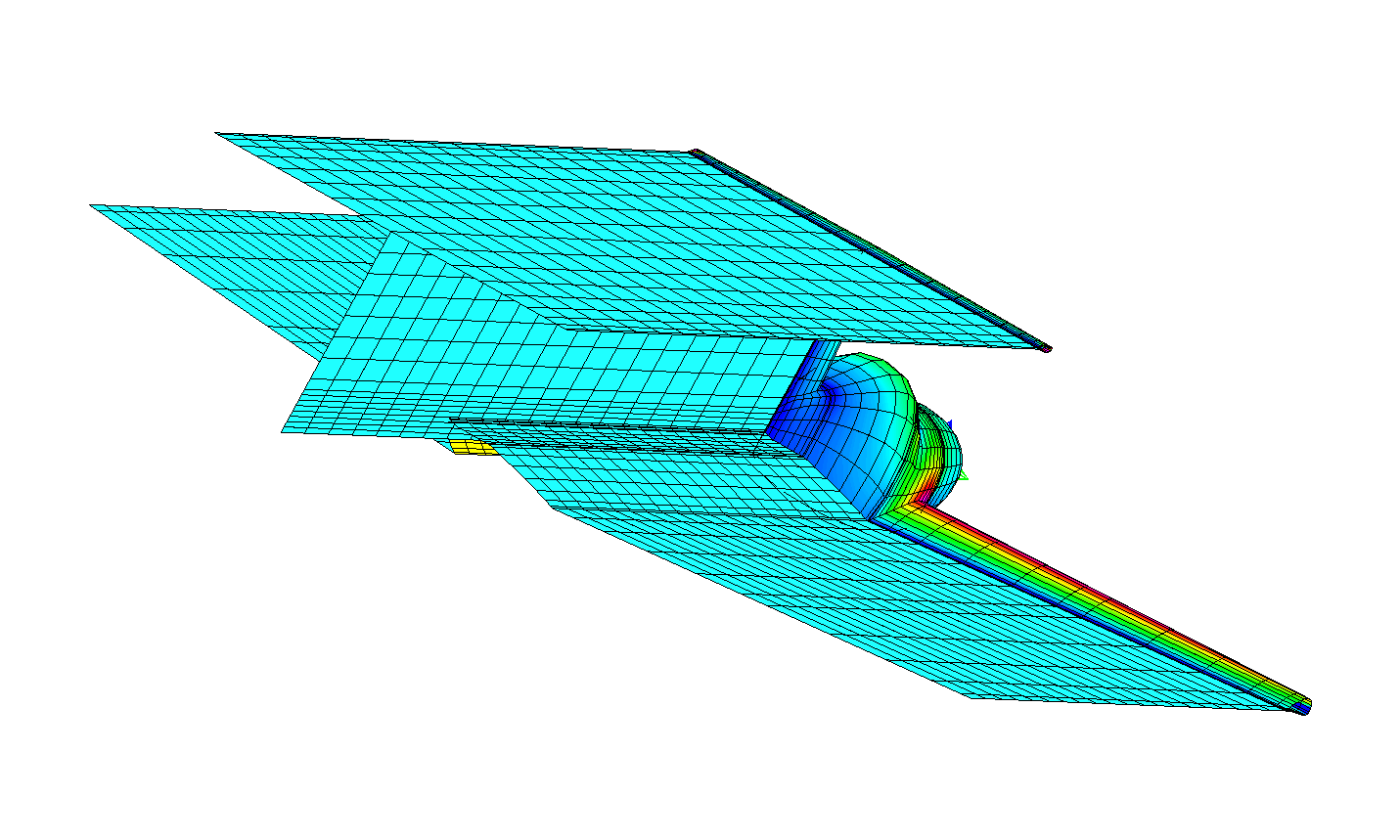
Postmarc is a graphic postprocessor for Cmarc and Pmarc-12 output files. It has a simple, intuitive, and self-documenting user interface. Postmarc provides rotatable and zoomable views of the model and its wakes, with color mappings of pressure, velocity, Mach number and an array of boundary-layer parameters; vector arrows representing local velocities on the model surface and in the surrounding free stream; pressure distributions along any cross-section; and on- and off-body streamlines and velocity scans. On-body streamline displays include boundary layer analysis. Data may be displayed for a single output file or for the difference between two output files for the same model (for example with different angles of attack). Rectangular and cylindrical scan volumes can be displayed in several ways, including spectrum-plotted planes slicing the flow field at multiple locations. Routines for calculating center of gravity, moments of inertia, and bending, shearing and torsion loads on flying surfaces are included.

Wakes

Both the initial geometry and animation of time-stepped wakes may be displayed.

This example shows the wake curl up off a wing tip at 5 degrees angle of attack in a GIF89A animation.

Integrated forces and moments

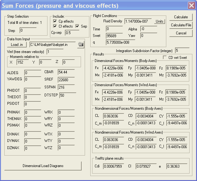Forces and moments for body and wind axes, derived from the OUT file, are diaplayed to allow rapid evaluation and comparison between baseline values obtained from the Trefftz plane analysis and those obtained from integrating pressures over the model. This comparison, along with XY plots of variables over a range of time steps, provides a measure of the stability and probably accuracy of the solution.

Contouring control

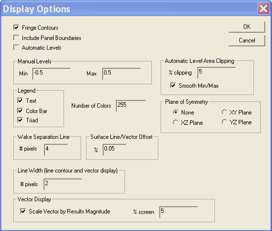The first button in the contouring group is the contouring/display setup form. In this form the user sets options pertaining to the display.

To begin with, the user can choose the number of colors; the maximum is 255. The range of values to which the spectrum maps may be set by the user or automatically. The useful range for pressure coefficients is from about -1.5 to 1.0, though the band from -0.5 to 0.5 may be of greater practical interest, and is the default. The useful range of velocities is from 0 to 2.0 or so. Other parameters, like skin friction, have other ranges.

Automatic selection is most useful if the input data are free of spurious highs and lows. This is seldom the case. It is handy, however, for targeting the appropriate range when a number of different parameters, like skin friction coefficient or boundary layer thickness, are being examined.

Spectrum plots may be smoothly contoured ("Fringe contours" on) or each panel may be solidly colored, reflecting the raw data. Fringe contours produce a more realistic and intuitively meaningful display.

Panel edges may be displayed or omitted.

Symmetrical half-models can be mirrored about any of the three orthogonal planes. The reflection plane of interest is usually the XZ.

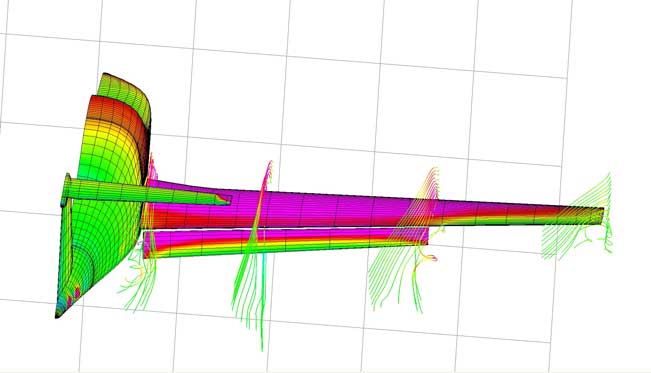
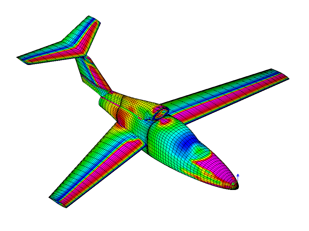
Cp, pressure coefficient

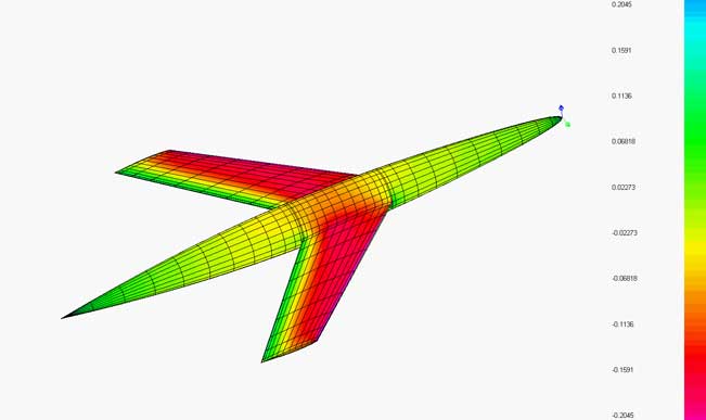The spectrum plot option depicts pressure distribution on the surface of the body.

Surface flow vectors

The vector ("XYZ") button causes the surface flow velocity for each panel to be displayed as an arrow on a hidden-line depiction of the body. The direction of the arrow indicates flow direction and its color represents the speed of the flow. The length of an arrow does not represent the magnitude of velocity; arrow are sized to fit within their panels.

To enhance the visibility of arrows, the color of the model can be set by selecting View > Solid color from the pull-down menus.

Pressure cross-sections

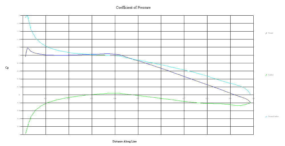Once a color "spectrum plot" has been drawn, the user may drag a line anywhere along an orthogonal view of the geometry and a 2D graph will be generated of the Cp (pressure coefficient), Vm (velocity magnitude) or M (mach number), whichever was displayed, on both near and far surfaces along the length of the line.

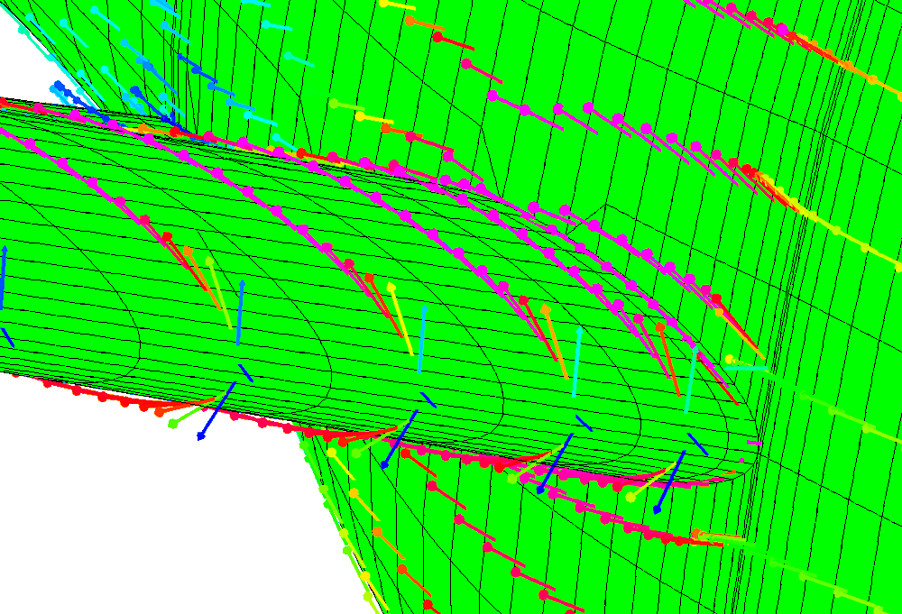
On-body streamlines and boundary layer analysis

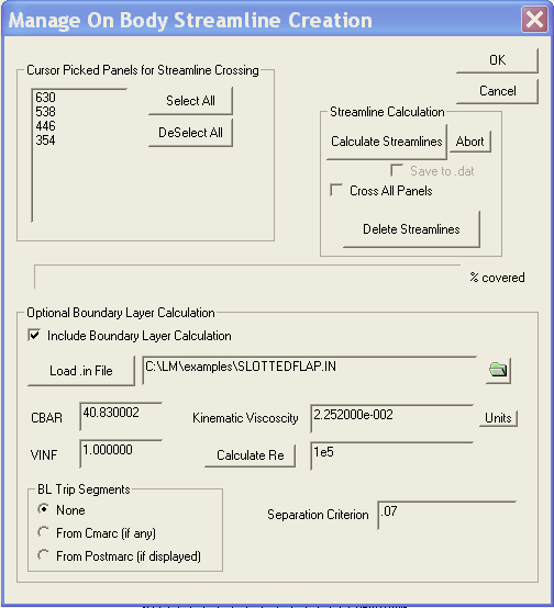The paths of streamlines can be displayed in relation to the body. On-body streamlines originate from the centroids of specified panels. Off-body streamlines originate from points in the space surrounding the model. Lines are color-coded to indicate local flow velocity.

Unlike Pmarc-12, Postmarc does not require re-running a full analysis for each new set of streamlines, veclocity scans, etc.

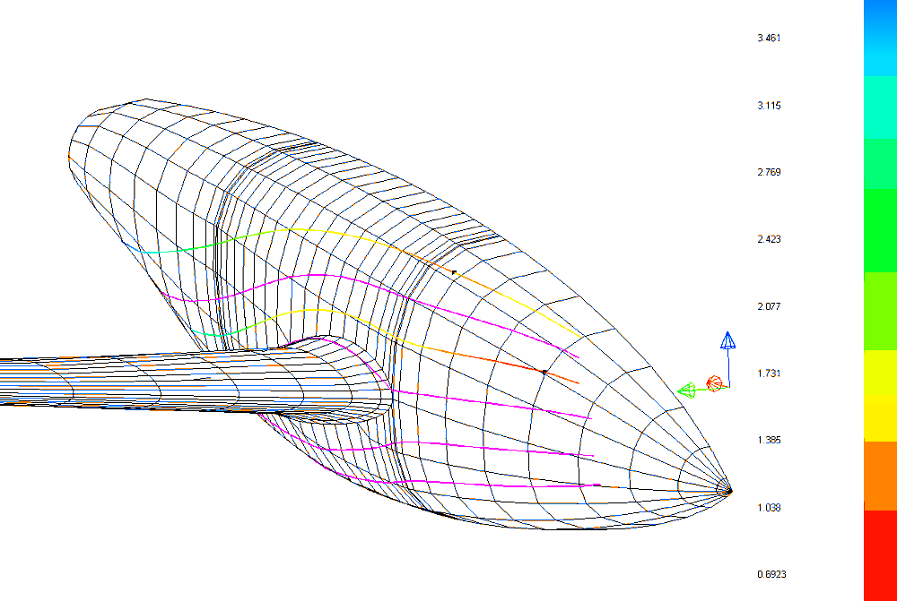In this example, boundary layer thickness is mapped by color along several on-body streamlines. Black diamonds mark locations where transition from laminar to turbulent flow was detected. Streamlines terminate when turbulent separation occurs.

Off-body streamlines

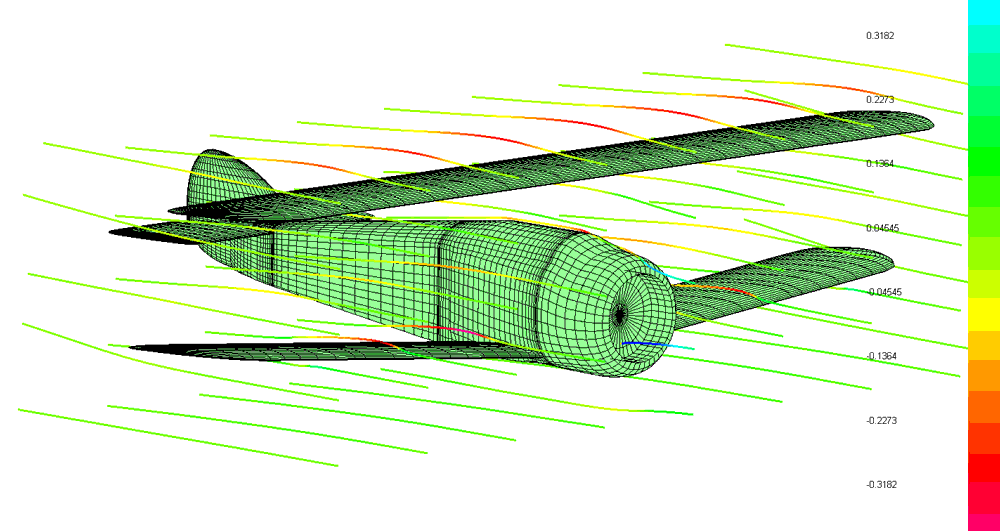Coloring of off-body streamlines may encode coefficient or pressure, velocity magnitude, or Mach number. Streamlines may form a regular rectangular or cylindrical grid, or may originate at arbitrarily sepcified points.

Off Body streamline locations can be cursor-selected for detailed study of areas of special interest.

Rectangular and cylindrical velocity scans

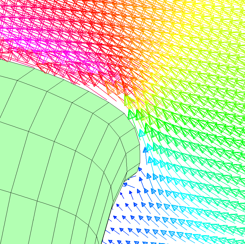Flow velocity and direction may be displayed at grids of off-body points defined in the input file. Here, flow approaches the NACA cowl lip of a T-6 Texan.

Boundary layer

If the model has been automatically "coated" with streamlines, a number of boundary-layer characteristics, including skin friction coefficient, boundary layer thickness and form factor, and laminar or turbulent state, can be spectrum-plotted over the model surface, and an estimate of viscous drag can be made.

Differencing

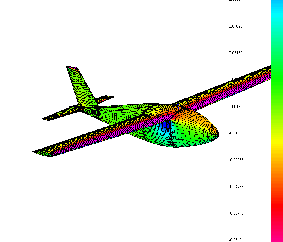Postmarc will map the differences in Cp, Vm, and Mach between two models. The models must be identically paneled, but can differ in dimensions and/or in flight conditions such as angle of attack or Reynolds number.

After you select two models and the Boolean operation (second-minus-first, first-minus-second, addition or none) to be performed, all commands related to pressure, velocity, and Mach number (including pressure distribution graphs, but not including XYZ plots) relate to the two files together.

The image shows pressure changes resulting from a change of one degree in angle of attack. Note that the changes are small, and so the automatically selected spectrum range is much narrower than usual.